Machine Learning: An Introduction
ChatGPT, to some a curse, to others a blessing. While it may be among the intrepid student’s most valued tools and the bane of a teacher’s career, ChatGPT has become among the most prominent symbols of recent progress in computer science. Over the past few years, the development of artificial intelligence programs and tools have revolutionized Internet searches while making information acquisition increasingly convenient. In part due to these emerging search engines, artificial intelligence has launched to the forefront of technological development, scientific investigation, and legal qualms. While readers are likely familiar with ChatGPT and the convenient artificial intelligence assistants integrated in Google and Microsoft search engines, these only represent the very tip of the AI iceberg. Along with revolutionizing our daily lives and learning experiences, artificial intelligence has brought about significant changes in scientific research. Its integration into numerous fields has led to the development of increasingly effective, timely, and inexpensive research strategies and provided entirely new avenues of exploration.
Machine learning has been among the most popular applications of artificial intelligence to diverse areas of research. Generally speaking, machine learning is a field of computer science focused on developing algorithms and computational models that are able to make predictions about an unknown dataset. The most distinctive aspect of machine learning is the aspect that lends it the very name ‘machine learning’: the ability to learn. Machine learning algorithms are designed to constantly adapt to new inputs to make increasingly accurate predictions. The ability to make changes to its parameters and focus allows a machine learning algorithm to become a potent predictive tool that can often outperform other kinds of mathematical models.
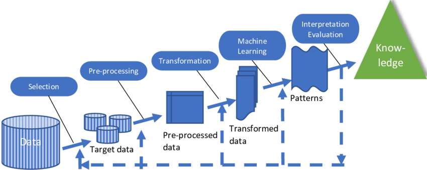
A basic diagram of the machine learning process starting from acquisition of the dataset to interpretation of the final output of the model. Image credit: (Huffmeier et al., 2020).
The diagram above outlines the basic procedures that are applied when using a machine learning algorithm. Oftentimes, the process begins when a machine learning model is selected that will best serve the needs of the researcher. There are a wide variety of machine learning models available, each having different strengths that cause them to be better suited for different applications. We will explore a few different machine learning models later in the lesson. The basic workflow of a machine learning project is detailed below:
-
The first step of a machine learning project is to choose a data set. Datasets come in many formats and can be of varying quality depending on the collection technology and costs. Researchers must select datasets that can conform to the chosen algorithm and provide meaningful insights into the research question.
-
The learning phase forms the core of machine learning and is what allows algorithms to make effective predictions. The model feeds the dataset through the algorithm and evaluates the results. Based on these results and comparison to known values, the model is adjusted over several iterations to achieve increasingly accurate results. The augmented model is then used to make predictions about a novel dataset to which it has never been exposed.
-
When the dataset is fed into the machine learning model, it must be altered to be understood and augmented by the computer. The dataset, which can consist of numbers, letters, or images is converted into sets of numbers or variables that can be readily interpreted by the model. Such sets are subjected to transformations so they can be fed through the mathematical algorithm that forms the core of the machine learning model.
-
The algorithm is run until it is able to produce sufficiently accurate predictions or until changes must be made by the researcher. The results of the algorithm, which can take the form of similarity comparisons, phylogenetic trees, and structure prediction, are then evaluated and used for further research applications. In the case of many machine learning algorithms, models that can produce accurate results are used to draw conclusions from new datasets.
Machine learning is a complex field and the steps above are an oversimplification of the entire process, but they give a general idea of how research is conducted using machine learning algorithms. Now that we’ve looked at a basic outline of the machine learning process, let’s take a deeper look at the learning aspect.
Learning Pathways
All machine learning algorithms employ some version of learning, a process that allows them to make increasingly accurate or useful predictions from a dataset. However, there are several different methods of learning that can be applied depending on the aim of the research and the composition of the data. Below we’ll explore a few of the learning methods commonly used in machine learning.
Supervised Learning
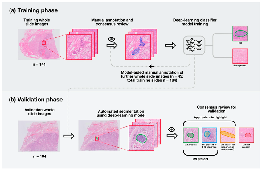
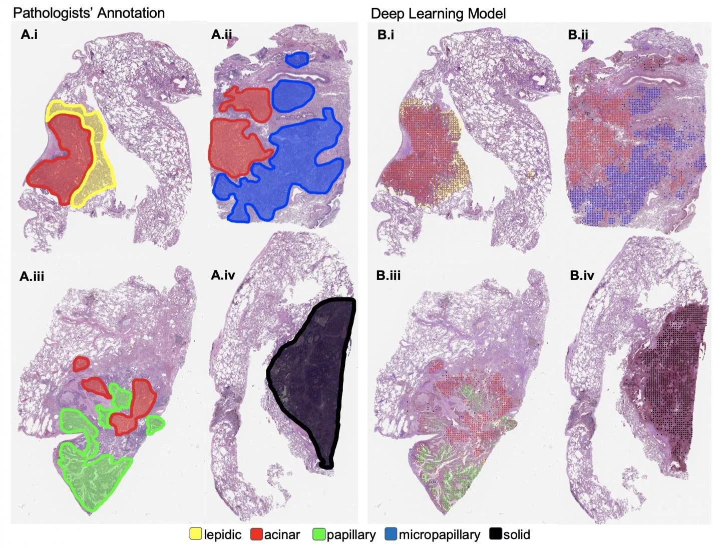
Supervised learning is among the most common types of learning used in machine learning. In supervised learning, the machine learning algorithm is given an initial dataset, known as a training dataset, that includes the information needed for the algorithm to make proper augmentations. When performing supervised learning, the process begins with analysis of the training dataset. The training dataset can come in many forms depending on the data format used, but it generally consists of data that has marked the features that the algorithm is being trained to identify. As an example, suppose that a machine learning algorithm is being trained to diagnose esophageal cancer based on images taken of the esophagus. In this case, let us assume that a certain raised area on the esophageal tissue is often associated with malignant tumors. In a training dataset, a medical professional would annotate images with highlighted boxes or another method to mark cases where the raised area is present. When given the training dataset, the machine learning algorithm would make changes or ‘learn’ based on the characteristics of the images that have been identified as having or not having the raised area associated with cancer.
A diagram of annotated samples of cancerous tissue and machine learning predictions. Image credit: (Ghosh et al., 2021).
Annotated training dataset and machine learning predictions for lungs affected by cancer. Image credit: (Hassanpour, 2019).
Clearly this is only one example and there are various methods of annotation that can be used depending on the chosen dataset and format. The algorithm makes predictions based on the images provided in the training dataset and makes augmentations until its predictions are close to the annotations themselves. In the case of the cancer example, the algorithm would appropriately identify the presence/location of an upraised area in the esophageal images. Once its predictions are sufficiently accurate, the machine learning model is exposed to new datasets. Successful learning has taken place when the algorithm can make accurate predictions when given the new dataset.
Unsupervised Learning
While supervised learning and the use of a training dataset is among the most frequently used learning pathways in machine learning, it is not always applicable to every situation. At times, a dataset may be too large to be feasibly annotated manually or training data may not be available. In this case, a training dataset is not used in a method known as unsupervised learning. Rather than feeding the algorithm an annotated dataset for learning, unsupervised learning relies on the algorithm’s ability to identify inherent patterns, characteristics, or features within the dataset. Generally, the algorithm searches for similarities among datasets or components of the dataset and identifies these as key characteristics that can be used for predictions. As an example, imagine that the genomes of two closely related organisms have been sequenced and the researchers desire to find homologous sequences, or sequences that were present in the common ancestor. An unsupervised learning algorithm would identify similarities between genetic sequences, and, as such, it could be used to find segments of DNA that are identical and likely to be homologous.
A visual representation of semi-supervised learning that depicts a mathematical model and a similarity grouping. Image credit: Avi Bewtra.
A comparison of supervised learning (finding specific trends from training data) and unsupervised learning (finding shared characteristics among raw data). Image credit: Aidan Wilson.
Semi-Supervised Learning
As the name implies, semi-supervised learning is a learning pathway that is situated somewhere between supervised and unsupervised learning. Semi-supervised learning often borrows from characteristics of the other two learning pathways to create more effective models. Oftentimes semi-supervised learning will employ training datasets as a supervised learning algorithm would, yet these will lack key labels or will have missing information. The presence of a training dataset allows the algorithm to learn from previously annotated data, but the lack of certain information necessitates the use of pattern searches characteristic of unsupervised learning. The combination of supervised and unsupervised learning in semi-supervised learning can be used to create more effective machine learning algorithms by incorporating the most potent characteristics of the two distinct learning pathways.
Models: Diverse Approaches to Machine Learning
Just as there are multiple ways in which a machine learning algorithm can learn, there are also diverse models used as the basis for machine learning algorithms. While all models operate on the same premise of training an algorithm to make decisions and produce increasingly accurate results, they operate under various different principles. Some models are relatively simple with few layers while others are highly complex, possessing multiple layers and often termed deep learning algorithms (deep learning is primarily a reference to the presence of multiple layers of processing). Let’s explore a few examples of models commonly used in machine learning.
Artificial Neural Networks
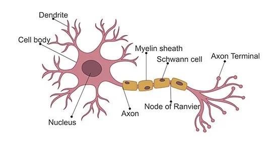
Artificial Neural networks (ANN) were once at the forefront of artificial intelligence research, though they have fallen to the wayside in that particular research in favor of other methods. However, ANN remain prominent in machine learning research and can be used for diverse applications within the field. In their simplest form, ANN are digital representations of the basic workings of an organic brain. ANN are composed of subunits known as nodes that are designed to mimic the neurons in a brain. The nodes are connected to each other by artificial ‘synapses’ and communicate with one another. ANN can be relatively simple with one layer or they can become very complex with multiple layers of nodes, each with a designated function. In more complex networks, one layer may be responsible for receiving inputs such as the raw dataset. This is transformed by the nodes which communicate information to one another. Based on what information is sent from node to node and which information is withheld, the ANN adapts its algorithms to make more accurate predictions.
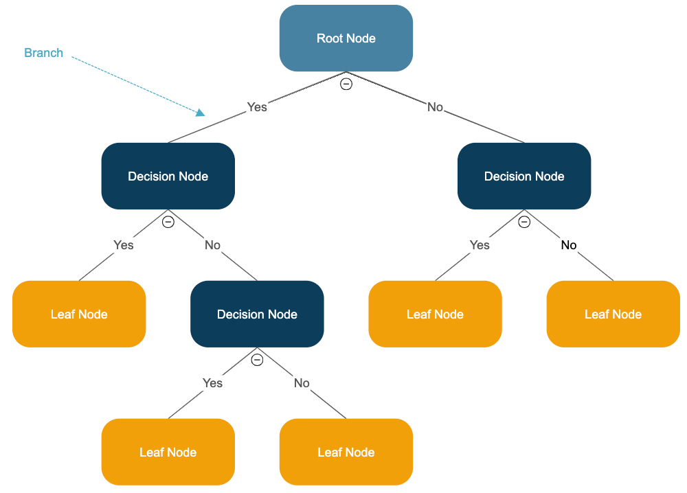
A basic schematic of decision trees as used in machine learning. Image credit: Smartdraw.
Regression Analysis
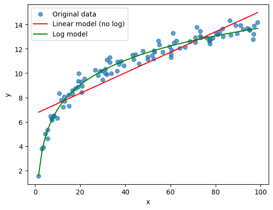
While the two previous models have either attempted to model organic brains or the decision-making process, regression analysis relies almost wholly on statistical methods. Regression analysis employs statistical algorithms to find functions and mathematical models that serve as the best fit for a given dataset. They can be extremely simple, with models such as linear regression simply finding a linear model that best accommodates the information in the dataset. However, they can become considerably more complex with models that employ higher order mathematics and that may have multiple layers or steps. In addition to linear regression, polynomial, logarithmic, exponential, and many other models can be adjusted to fit a dataset.
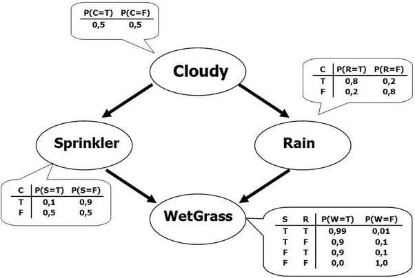
A basic schematic of a Bayesian network. Image credit: Devin Soni.
The nodes within artificial neural networks seek to imitate neurons in organic brains. Image credit: CusaBio.
Decision Trees
Decision trees are among the simpler models used in machine learning, though they can be used to great effect. As the name implies, Decision Trees generally take the form of a branching tree starting from the raw data and branching off in a continuous fashion. These models vary in complexity depending on the application, but branches typically appear when certain characteristics of interest differ between components of a dataset or components of different datasets. Based on the characteristics that are present in the specific data point or set that an algorithm is analyzing, it will choose a particular path on the Decision Tree. By following these paths and continuously adapting the tree and its algorithms, the machine learning algorithms is able to draw conclusions or make more and more accurate predictions.
Logarithmic and linear regression models for dataset. Image credit: Juan Estaban de la Calle.
Bayesian Networks
A Bayesian Network is a somewhat more abstract model of machine learning that relies on complex graphs that lack a cyclic nature. Generally, Bayesian networks are self-contained models that rely on conditional probabilities based on two or more variables and express these through the use of the aforementioned graphs. As an example, Bayesian networks can often be used to model symptoms of a certain disease or diseases and estimate the probabilities that individuals have a disease based on their symptoms. Since the symptoms may be caused by more than one disease or by a confounding variable, the model relies on conditional probabilities to calculate the most likely outcome or possibility.
Activity: Understanding Regression Analysis
Regression analysis is a commonly used model in machine learning that relies largely on statistical methods. While regression analysis can become complex, particularly when higher order functions or multiple steps or dimensions are involved, some analyses are relatively simple from a mathematical standpoint. At its simplest, regression analysis can take the form of finding a line of best fit (or linear regression model) for a dataset that can be represented as a set of points on a 2-dimensional coordinate plane. To better understand regression analysis, an important model in machine learning, let’s perform a simple mathematical exercise involving regression.
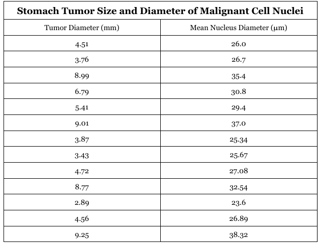
Suppose that a researcher is studying cancerous tumors found in the stomachs of a set of patients. To learn more about cancer development and the characteristics of the malignant cells, the researcher hopes to determine whether there is a relationship between the size of the stomach tumors and the diameter of the nucleus of the malignant cells. Previous research has shown that the nuclei of cancerous cells can be abnormally large, so the researcher predicts that there may be a relationship between tumor size and the size of cancer cell nuclei. To test this mathematically, the researcher has compiled a dataset of 13 tumors consisting of tumor diameter measured in millimeters and the mean diameter of the cancerous cells contained within (measured in micrometers). Below is a table containing the data that the researcher intends to manipulate.
Table consisting of the diameters of 13 stomach tumors and the mean diameter of the nuclei of the malignant cells.
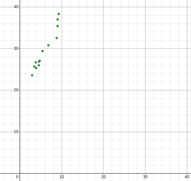
When creating a regression model, it is best visualized if it is placed alongside the data points on a coordinate plane. Below is a representation of the thirteen data points on a coordinate plane without a regression model.
The thirteen data points represented on a coordinate plane. Graph created using Desmos.
Many graphing calculators including the Desmos Online Graphing Calculator contain a built-in function that can be used to generate linear regression models. While these are convenient and far more practical than manual calculations, we will manually calculate the equation of a regression line to better understand the process undertaken by machine learning algorithms when given a dataset. Regression models are also known as least squares models a term that refers to their goal of minimizing the squared distance between the actual data points and the nearest point on the regression model. When considering the term least squares, it should make sense why we would wish to minimize the distance between the individual data points and those contained in the regression model. If this distance is minimized across all data points, the model is the closest it can possibly be to the data itself and thus serves as the best possible model of its kind. However, one may be left wondering why it is called a least squares model. When creating a regression model, the distance between the data points and the closest point on the model (known as residuals) can be positive or negative depending on whether the actual data point is above or below the model. The presence of positives and negatives interferes with the process since opposites cancel. As such, residuals are squared to make all values positive. This lends the name to least squares models. Now that we’ve had a brief overview of what a regression model is, let’s do a little math!
As readers have learned in previous math classes, the equation of a line can generally be expressed as y = a + bx. As lines, linear regression models must follow this same format. As a result, we must only find the values of a, the y-intercept of the line, and b, the slope of the line, to create our equation and generate a graph of the model. To begin, let us grant ourselves an easy starting point by finding one point that is guaranteed to be on the least squares linear model. This point is the average of the x values (in this case tumor diameter) and the average of the y values (in this case average nucleus diameter). Try to find this point and reveal the answer to check your work.
-
To calculate the mean of each coordinate, you must add each of the individual values and divide the sum by the total number of values. For the x values (tumor diameter), the setup would be as follows:
(4.51 + 3.76 + 8.99 + 6.79 + 5.41 + 9.01 + 3.87 + 3.43 + 4.72 + 8.77 + 2.89 + 4.56 + 9.25) / 13
-
(5.84, 29.60)
Now that we’ve found one point guaranteed to be on the graph of the linear regression model, let’s find the values that define the equation of the line. To begin, we will find the more complex of the two values, b, or the slope of the line. The slope of the least squares regression model is computed using the following formula:
Formula for the slope of a least squares regression line. Image credit: Technology Networks Informatics.
The above formula may seem very daunting at first, but it is quite easy to work with once it has been broken down into smaller pieces. Starting with the numerator of our fraction, we have the summation of (x - x̄) multiplied by (y - ȳ). The first factor within the summation are the differences between the x values (or tumor diameters) and the mean of the x values or the mean tumor diameter (denoted as x̄). In the previous step we calculated the mean values of the x and y values and these can be substituted in for x̄ and ȳ. The mean is subtracted from each of the 13 tumor diameters listed in the table and multiplied by the difference between the corresponding y-value and the average y-value. Following this process, one should obtain 13 products that are added together to obtain one value for the numerator. Moving to the denominator of our formula, we can see that there is a single term that appears very similar to the first factor in the numerator. They are nearly identical, except that each difference between the x-values and x̄ is squared before they are added together. Then we must only multiply the two factors in the numerator and divide by the summation we obtain in the denominator to get our slope, or the value of b in our linear equation. Try to calculate this yourself and check your answers below.
-
First we begin by calculating the summation in the numerator of our formula. The summation is calculated as follows: (4.51-5.84) (26.0 - 29.6) + (3.76 - 5.84) (26.7 - 29.6) + (8.99 - 5.84) * (35.4 - 29.6) ....
For the denominator the same process is repeated with the values corresponding to the x-coordinates, except that each difference is squared and they are directly added to one another. The mathematical setup is as follows: (4.51-5.84)^2 + (3.76 - 5.84)^2 + (8.99 - 5.84)^2 ....
-
Σ((x - x̄) * (y - ȳ)) = 133.98
Σ(x - x̄)^2 = 68.65b = 133.98/68.65 = 1.952
Now that we’ve successfully calculated the value for b, the slope, we now only have one variable left to determine: a. Since we have values for all of the remaining variables in the equation y = a + bx, we can simply solve for a. You know that we have a value for b, but you may ask how we can have values for x and y since we cannot be certain that any of the raw data points are on the graph of the line itself. This is true, but in step 1 we calculated the coordinates of one point that we know must be on our linear model. By substituting these coordinates for x and y and plugging in our value for b, we can use basic algebraic techniques to solve for the y-intercept a. Try to solve for a and plug in the values to obtain the equation of the linear regression model. Check your answer below.
-
We know that the equation of our line will follow the form y= a + bx and we know that our b-value is 1.952 from the previous step. With this knowledge, we can obtain the following setup: y = a+ 1.952x.
With the point that we calculated in the first step (5.84, 29.6), we can substitute for x and y. Plugging in these values leads to the following equation: 29.6 = a + 1.952(5.84).
With some simple algebraic manipulation, we can isolate a and end up with the following equation: a = 29.6 - 1.952(5.84).
Having found the value of a, we can simply plug in the numerical values of a and b to find the equation of our linear regression model.
-
a = 18.20
y = 18.20 + 1.952x
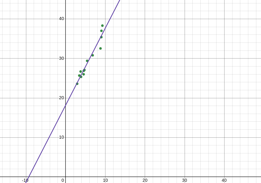
Having our linear regression model, we can plug the equation y = 18.20 + 1.952x into a graphing calculator to visualize the graph. This is best done when the data points are also plotted on the same coordinate plane. Below is a graph showing our newly constructed linear regression model among the data points shown in the table above.
A coordinate plane showing the data points from the table and the linear regression model that was created. Graph created using Desmos.
From the graph above, it can be seen that the linear regression model captures the trend in the data quite nicely and shows a strong positive correlation between tumor diameter and the average cell nucleus diameter. In addition to capturing the trend in the data, regression models such as the linear model shown above possess predictive power. If a strong correlation is established between two variables as it has been in the dataset above, the model could possibly be used to make predictions about values outside of the dataset. These predictions, known as extrapolations, can be relatively accurate if the model is a very good fit. As an example, if the researcher wished to know what the average cell nucleus diameter of cells within a tumor with a diameter of 40 mm, they could use the regression model to predict this value. Machine learning algorithms performing regression analysis use techniques akin to those we performed above, though they tend to be more complex with many more steps. However, the principle is largely the same as the algorithm searches for a model that best fits the data and adjusts it to make accurate predictions beyond the scope of the dataset.
Machine Learning in Computational Biology
We have explored the basic principles of machine learning and delved into some of the distinct learning methods and models that are commonly used in the field. Even so, one may still wonder how machine learning can be applied to computational biology. Some applications of machine learning in biology were hinted at above, but the field of machine learning has proved instrumental to advancements in computational biology. The use of self-adjusting algorithms has allowed for far more effective data processing and the development of models that can make more accurate predictions than most others known. Additionally, machine learning has made computational biology far more accessible as it has reduced the need for wet lab work and can be relatively inexpensive. Let’s take a look at a few specific areas of computational biology that have seen a notable rise in the use of machine learning.
Phylogenetic Trees
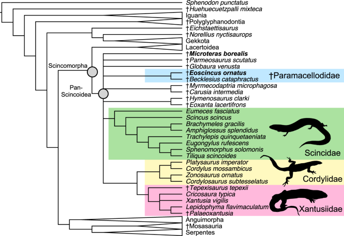
Machine learning has become key to divining the evolutionary relationships between organisms and tracing their shared ancestry through time. A key way scientists use to express evolutionary relationships are phylogenetic trees, diagrams that visually display how organisms diverge from a common ancestor. A quick look at a few professional phylogenetic trees will quickly reveal their complexity, and the sheer number of taxa included in many hint at a very large amount of data. Computational biologists often use machine learning algorithms to construct phylogenetic trees. Whether given genomes or morphological characteristics, machine learning algorithms can search for similarities between various organisms to make predictions about their evolutionary relationships. Efficiently working through large datasets, machine learning models can effectively generate phylogenetic trees that often have a relatively high degree of confidence. These phylogenetic trees are used to study the evolution of extinct organisms, develop vaccines against viruses, and learn about human origins.
DNA sequences are analyzed using genetic algorithms to find favorable genotypes.
Structure & Function
As readers have doubtlessly heard in a biology class, biological entities have structures meant for their specific functions. This is the case for all biological structures, including the complex and diverse array of proteins that power cellular metabolisms. Proteins are very complex structures often consisting of hundreds of amino acids that experience different interactions depending on their orientation and molecular composition. The complexity of proteins can make them very difficult to model, making protein modeling yet another challenge that machine learning has been set to tackle. Computational biologists have developed machine learning algorithms that can analyze the sequence of amino acids in proteins and predict the interactions they will have with one another. Based on these predicted interactions, the algorithm can develop plausible structures of the protein until it settles on what appears to be the most plausible structure. The ability to accurately predict protein structures is instrumental to the fields of medicine, cellular biology, and biochemistry.
A phylogenetic tree of lizards, snakes, and related reptiles. Image credit: (Brownstein et al., 2022).
Genetic Algorithms
Genetics, the study of inheritance through DNA, is among the key disciplines within the field of biology. Significant progress in DNA sequencing technology has considerably reduced the cost and time involved in generating complete genomes from desired organisms. While genomes are available, the long strings of As, Ts, Cs, and Gs, are often so large that they are difficult to manage. The size of these datasets and the great possibility of human error have led to the development of specialized machine learning algorithms designed for genetics applications. These models, known as genetics algorithms, are geared toward finding specific genotypes to use for solving problems in the real world. Genetic algorithms operate on principles similar to natural selection to accurately mimic the inheritance of genetic material from generation to generation. The use of a specific algorithm allows for the relatively rapid generation of a large amount of genotypes in the search for the specific one that is desired.
3-dimensional structure of a protein. Image credit:Brown University.
Since its humble beginnings in artificial intelligence research, machine learning has come a long way and become an invaluable tool in scientific research. Computational biology relies heavily on diverse approaches, learning styles, and models of machine learning to solve real-world problems and expand our understanding of the natural world.

